4.6. Segmenting cells from a 2D image and automated cell classification

Figure 1: Cross-section of a hypocotyl of A. thaliana at 14 days
In this section, we are going to see how we can extract the 2D shape of cells from a 2D image of the cross-section of a hypocotyl of Arabidopsis thaliana, and see how we can train a cell classifier to automatically label cell types. This tutorial is based on [BarbierDeReuille.Ragni.InPress]. To start, download this dataset, provided by Dr. Laura Ragni.
4.6.1. Pre-processing
Although the image is of very good quality, the cells contain a lot of small “objects” that may cause problem when segmenting. In this sense, an object is a contiguous group of pixels whose intensities are all strictly greater and strictly smaller than their neighbors. For the pre-processing, we will remove them:
Load the image
Col_14d_63x_bl1_4sti_s1.ome.tiffChange the transfer function to
Scale Grayand auto-adjust its range.Re-scale the stack’s intensities to maximize its dynamic range:
Process [Stack]Filters/Apply Transfer Function Filter the stack using two gaussian blurs with a very small radius (about the half voxel size):
Process [Stack]Filters/Gaussian blur Parameter Value X Sigma (μm) 0.1 Y Sigma (μm) 0.1 Z Sigma (μm) 0 Remove all the small objects from the image. This process will remove any object (see above for the definition) whose area (for a 2D image) or volume (for a 3D image) is smaller than some threshold. Note that the shape of the object is irrelevant. As the smaller cells are about 3-4 μm², set the size to 2 μm²:
Process [Stack]Morphology/Sieve Filter Parameter Value Size (μm²) 2 Save this stack as it might be useful later.
4.6.2. Segmentation of the vascular tissues

Figure 2: Segmentation of the vascular tissues
Use the
Segment Sectionprocess in theSegmentationfolder. This process will blur the cells slightly and use the auto-seeded watershed for the segmentation itself. The auto-seeded watershed requires the cell walls to be bright and the background to be dark, which is the opposite of our images here. The last option of the process is to invert the image before segmentation. Otherwise, use the default options.Process [Stack]Segmentation/Segment Section Parameter Value BlurX 0.3 BlurY 0.3 Invert Yes We now need to remove all the segmented parts outside our region of interest. In the image, the vascular tissue is contained in a disc of radius 80 μm:
Process [Stack]Segmentation/Remove Labels in Shape Parameter Value Shape Sphere Center 0 0 0 Size 80 Create a cell mesh from the segmentation with a fairly fine description of the cell:
Process [Mesh]Cell Mesh/Cell Mesh from 2D Image Parameter Value Edge Length (μm) 1 To inspect the segmentation, it is simpler to show the outline of the cells. For this, in the main tab, un-check the
Surfacecheck box and check theMeshcheck box. For the mesh, select to view the cells (in theviewcombo box) and hide the points.
4.6.2.1. Correcting the segmentation
With the cell outline visible, you can check the correspondance between the segmentation and the image. Segmentation errors can be broadly classified in three categories:
- Over-segmentation is when a single biological cell has been identified as many cells by the segmentation..
- Under-segmentation is when some biological cells have been identified as a single cell by the segmentation.
- Mis-segmentation is any error that doesn’t fall into either previous category.
4.6.2.1.1. Over-segmentation

Figure 3: Example of over-segmented cell.
Over-segmentations are the easiest error to correct.
- Show the segmented stack (which should be in the work stack)
- Using the 3D pipette, select the label of part of the cell
- Using the 3D bucket, replace all the other labels in the biological cell by the one selected.
- Re-create the cell mesh
4.6.2.1.2. Under-segmentation

Figure 4: Example of under-segmented cell.
Under segmentation is a bit more difficult as it requires local re-segmentation.
Erase the under-segmented cell.
Select the magic want and, in the view tab, in the
Stack
Editing
section, selectFillandNew Seed.Place seeds at the center of each biological cells.
In the menu
Labels & Selection, selectNew SeedUsing the 3D bucket, flood-fill the outside of the tissue. To flood fill an area, you need to press Shift and Alt while clicking with the left button of the mouse.
Swap the main and work stack:
Process [Stack]Multi-stack/Swap Main and Work Stacks Invert the main stack:
Process [Stack]Filters/Invert Swap the stacks back in place
Re-segment the image:
Process [Stack]ITK/Segmentation/ITK Watershed Delete the outside cell with the 3D bucket tool.
Re-create the cell mesh
Optionally you can re-invert the image by repeating steps 6 to 8.
4.6.2.1.3. Mis-segmentation
Correcting mis-segmentation is very similar to correcting under-segmentation. The only difference is that all mis-segmented cells should be deleted. Also, mis-segmentation is often due to issues with wall staining. If this is the case, place the seeds close to the cell wall to prevent the re-segmentation from “bleeding”“.
4.6.3. Automated cell classification
An automated classifier will try to identify cells from a set of adapted features. LithoGraphX offer a process computing a whole series of features adapted to cells segmented from 2D images. As often, cells will be identified by a numeric identifier, which you need to choose for each cell type. In this protocol, here are the identifiers we chose:
| Cell Type | Identifier |
|---|---|
| Xylem vessel | 3 |
| Phloem bundles | 4 |
| Cambium | 5 |
| Xylem parenchyma | 6 |
| Phloem parenchyma | 7 |
Creating the classifier is done in three steps:
- Label some cells by hand
- Compute the features
- Train the classifier
It will be important that all files linked to a given image share a common prefix.
4.6.3.1. Labelling of the cells
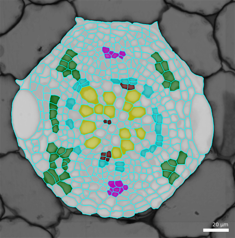
Figure 5: Example labelled cells.
Cells are labelled using the “parents” feature. Except that, instead of giving to a cell the id of its parent, we are going to give it its cell type identifier.
- Show the surface, selecting the
Parents - To see more easily, check the
Blendcheck box and decrease the opacity by moving the slider. - In the menu
Labels & SelectionselectChange current labeland enter one cell type identifier. - Using the 2D bucket, Alt-Left click on some of the cells of that identify
- Save the mesh file.
- Repeats steps 3 and 4 for each cell type, marking each time some of the cells and trying to mark as many of all the cell types.
4.6.3.2. Features computation
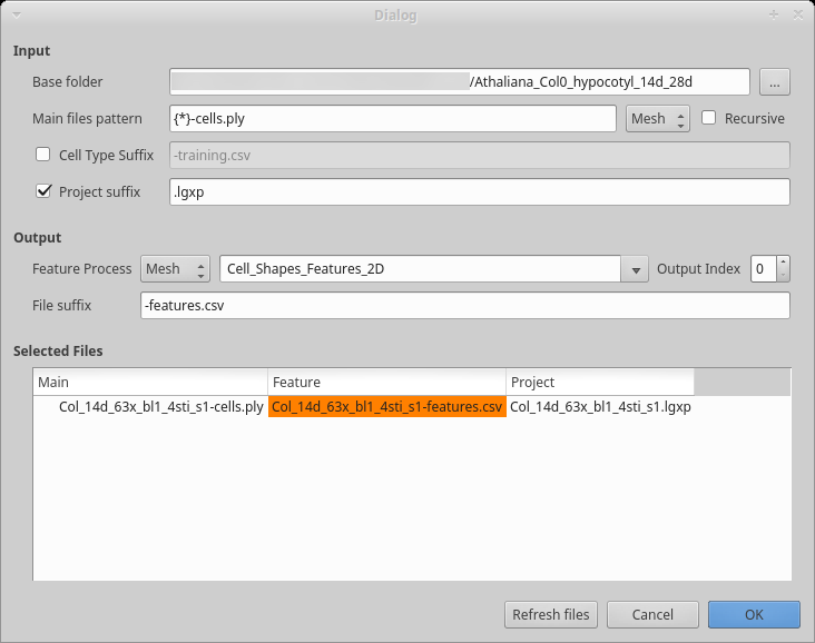
Figure 6: Dialog box to compute cells features.
Start the process creating the classifier features:
Process [Global]Cell Classifier/Generate Classifier Features If you have been editing all your files in the same folder, the base folder should be correct, otherwise, select the folder containing all your datasets. If you created separate folders for different datasets, check the
recursivecheck box.You may want to update the
Main file patternto reflect your convention. The base name is contained within the curly bracket and used as prefix for the other files. As you can see in the example, the mesh here also has a suffix.Inspect the file list to make sure all the files will be properly processed as you want. Then press the
OKbutton to start the process.
4.6.3.3. Training the classifier
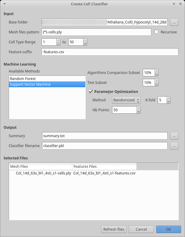
Figure 7: Creation of the cell classifier.
After having computed the features on all your samples you can train the classifier.
Start the process creating the classifier itself:
Process [Global]Cell Classifier/Generate Cell Classifier The input area works like the previous dialog box. You will notice the process allows you to use only a range of cell types. This can be useful if you are not sure about detecting some cell types.
We currently offer two algorithms: Support Vector Machine (SVM) and Random Forest. Previous tests showed that SVM work better for this particular problem, but you can select more than one algorithm.
After running the algorithm, you should examine the summary generated. You should in particular look at the confusions matrix and report at the top the file:
Machine Learning Summary
========================
Selected classifier:  Support Vector Machine

Testing using set with 9 elements
---------------------------------

Confusion matrix:
Predicted  3  4  5  6  7  Sum
Real
3          2  0  0  0  0    2
4          0  1  0  0  1    2
5          0  0  0  0  0    0
6          0  0  1  0  0    1
7          0  0  0  0  4    4
Sum        2  1  1  0  5    9

Classification report:
             precision    recall  f1-score   support

          3       1.00      1.00      1.00         2
          4       1.00      0.50      0.67         2
          5       0.00      0.00      0.00         0
          6       0.00      0.00      0.00         1
          7       0.80      1.00      0.89         4

avg / total       0.80      0.78      0.77         9


Score:  77.7777777778 %

Algorithms Details
==================

Support Vector Machine
----------------------

Best score with k-fold: 0.858823529412
Parameters:
class_weight : balanced
C : 31.04345899553238
gamma : 0.0514347955741465
4.6.3.4. Using the classifier
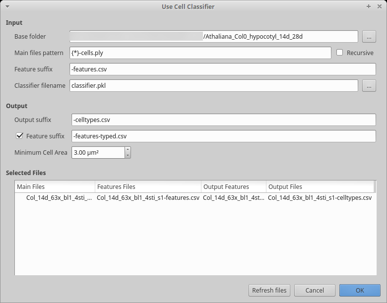
Figure 8: Using of the cell classifier.
After creation, we want to use the cell classifier:
Start the process to use the classifier:
Process [Global]Cell Classifier/Use Cell Classifier Choose the name of the classifier file you generated in the previous step
Fill in the input and output part as usual
In the output, the default is to write a CSV file containing two columns: the cell labels and the estimated cell type. You can optionally generate a file containing all the features and add a column with the estimated cell type. This file can conveniently be used for further filtering/analyses using R, Python, …
You can visualize the result by loading a mesh and changing the parents, using the files generated in the previous step (e.g. by default the ones ending up with
-celltypes.csv)Process [Mesh]Lineage Tracking/Load Parents
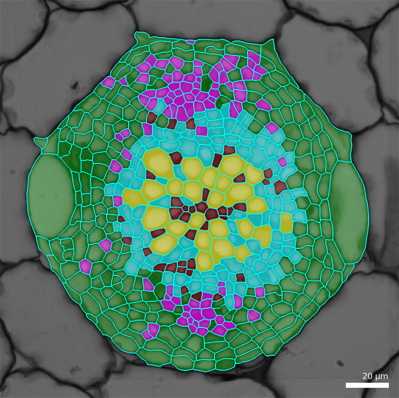
Figure 9: Result of the cell classifier.
| [BarbierDeReuille.Ragni.InPress] | Barbier de Reuille P, Ragni L. in press. Vascular morphodynamics during secondary growth. In: de Lucas M, Etchells JP, eds. Xylem: methods and protocols Springer. |